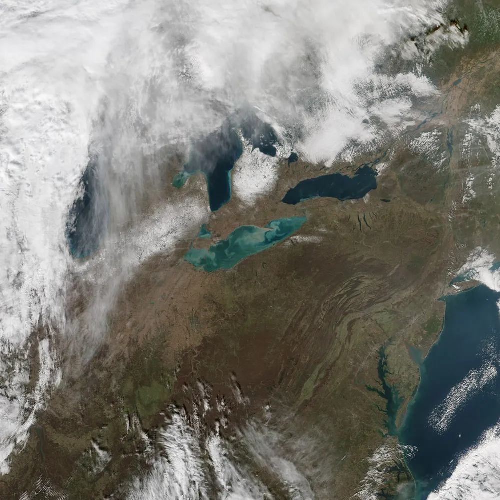
How Reliable Is Satellite-Derived Water Turbidity?

Satellite-derived turbidity can support reliable monitoring of sediment plumes, seasonal patterns and unusual changes across rivers, lakes and coastal waters. Its reliability, however, depends on whether the imagery, processing method and retrieval algorithm have been validated for the conditions being monitored. A convincing map is not enough: users need to know how closely the estimates match field measurements, where the method works and which observations should be excluded.

For project planning, the central question is therefore not simply whether satellites can measure turbidity. It is whether the resulting information is accurate enough for the intended decision—such as prioritizing sampling, tracking a dredging plume or assessing changes near a water intake.

Start by Defining the Water Quality Indicator

Water color, turbidity, suspended solids and transparency describe related but different properties. Treating them as interchangeable can produce a technically plausible result that does not answer the customer’s question.

Water color describes the spectral appearance of water. Sediment, algae and colored dissolved organic matter can all change it. A color change alone does not identify its cause.
Turbidity is an optical measurement associated with light scattered by material in water. Satellite algorithms estimate it from water reflectance through a calibrated relationship; they do not reproduce a turbidimeter’s measurement directly.
Total suspended solids or suspended particulate matter describes the mass of suspended material per volume of water, commonly expressed in mg/L. The relationship between this concentration and turbidity varies with particle size, composition and other properties.
Transparency or clarity describes how far light or a visible target can penetrate water. Secchi depth, measured in meters, is one common indicator. It is influenced by both light absorption and scattering and requires its own retrieval and validation.

Turbidity units also require attention. FNU and NTU refer to measurements made with different instrument specifications. They should not be assumed interchangeable across all waters. A project should record the field instrument, measurement method and reporting unit, then ensure that the satellite product is calibrated against a compatible reference.

If the operational need is to identify sediment-rich runoff, turbidity may be appropriate. If the requirement is sediment concentration, visibility or a specific contaminant, a turbidity map alone may not provide the required answer.

Why an Algorithm May Work in One Water Body and Fail in Another

Optical satellites measure reflected light across selected wavelength bands. The water signal depends on the combined effects of particles, pigments, dissolved substances and, in shallow areas, the bottom. Two water bodies with similar turbidity can therefore have different spectral signatures.

Some semi-empirical turbidity algorithms have demonstrated useful transferability across sediment-rich coastal and estuarine waters. The approach developed by Dogliotti and colleagues, for example, uses red reflectance at lower turbidity and near-infrared reflectance at higher turbidity to address reduced red-band sensitivity. Its validation used field measurements separate from those used to calibrate the algorithm.

This provides a sound starting point, but does not establish universal performance. A sediment-dominated estuary, an algae-rich reservoir and a shallow clear lagoon present different retrieval challenges. Published coefficients must also match the sensor’s spectral bands and the reflectance definition used by the algorithm.

Algorithm Selection and Applicability

Approach	Potential Fit	Conditions to Verify
Red-band retrieval	Sediment-dominated water within a validated low-to-moderate turbidity range.	Sensitivity at low values, saturation at high values, sensor-specific coefficients and local bias.
Red-to-NIR switching	Sediment-rich waters covering a wider turbidity range.	Band-switching behavior, weak NIR signals in clearer water and performance across the full local range.
Local empirical model	A defined water body with representative field measurements.	Independent performance on new dates, sites and seasons; avoid extrapolation beyond sampled conditions.
Multiband or machine-learning model	Optically diverse waters supported by sufficiently varied training data.	Overfitting, correlated training and test samples, and transfer to unfamiliar water types.
Transparency retrieval	Projects requiring Secchi depth or another defined clarity indicator.	Validation against the requested clarity measurement; do not substitute a turbidity-to-clarity conversion without testing it.

Image Processing Can Determine the Result

Atmospheric correction is a major source of uncertainty because the satellite receives light from the atmosphere and water surface as well as from within the water. Processing must isolate the aquatic signal accurately enough for the retrieval.

The joint NASA–ESA ACIX-Aqua assessment compared eight atmospheric correction processors using more than 1,000 field-to-satellite radiometric matchups. Performance differed among datasets and optical water types. This matters operationally: selecting a turbidity equation cannot compensate for unreliable input reflectance.

Check the algorithm’s required input before processing. Top-of-atmosphere reflectance, land surface reflectance, aquatic reflectance and remote-sensing reflectance are different quantities. In particular, water-leaving reflectance and remote-sensing reflectance can differ by a factor of π under the relevant convention. Substituting one for another without adapting the equation changes the result.

Stored pixel values also need the correct product-specific scale factor and offset. For example, USGS specifies a scale factor of 0.0000275 and an offset of −0.2 for Landsat Collection 2 surface reflectance. Those instructions do not automatically apply to another product or sensor.

Higher spatial resolution can help separate water from banks and resolve smaller plumes, but it does not guarantee better turbidity accuracy. Band placement, radiometric quality and aquatic processing remain essential. Hyperspectral imagery can provide additional spectral information, but still requires appropriate correction and validation.

Match Field Sampling to the Satellite Observation

A field measurement represents a location, time and sampling depth. A satellite pixel represents an area and an optically weighted signal from the upper water column. Validation must account for these differences rather than assuming that nearby observations are equivalent.

Define the decision and acceptable error. Specify the indicator, reporting unit, monitoring area and intended use. An alert for follow-up sampling may tolerate different uncertainty from a quantitative assessment near an operational threshold.
Choose representative stations. Cover relevant turbidity ranges, water types, seasons and plume gradients. Include open-water locations suitable for image matching. Keep shoreline stations where operationally necessary, but assess their mixed-pixel limitations explicitly.
Sample close to the actual acquisition time. Record coordinates, timestamp, time zone, depth, instrument and calibration checks. Choose the acceptable time difference according to local variability. Tidal fronts, storm runoff and dredging plumes may change too quickly for a same-day match to be adequate.
Record conditions that explain variability. Include rainfall, river flow, tide, wind, water depth and nearby activity where relevant. Repeated measurements or continuous sensors can help assess whether conditions changed around the overpass.
Screen the image and extract comparable observations. Exclude clouds, shadows, glint, bottom-contaminated areas and unsuitable shoreline pixels. A small pixel neighborhood can reduce noise in homogeneous water, but may mix different conditions across a plume boundary. Record its size and spatial variability.
Separate calibration from validation. Use one dataset to fit coefficients or select the model and reserve independent observations for evaluation. Holding out entire dates or stations can provide a stronger test of operational transfer than randomly splitting closely related observations.
Repeat across operating conditions. Evaluate performance during relevant seasons and events. If the available samples cover only a narrow range, limit the product’s claims to that range.

If a project needs suspended solids as well as turbidity, collect the appropriate laboratory samples. A local relationship between turbidity and suspended solids should be tested separately; it can change when the sediment source or particle characteristics change.

Troubleshoot Unexpected Results Before Issuing an Alert

Unexpected Turbidity Results: What to Check

Observed Pattern	Possible Explanation	Recommended Check
High values along banks	Mixed land–water pixels or light scattered from adjacent bright land.	Inspect the shoreline mask and image alignment; assess adjacency effects and the need for a justified exclusion buffer.
Bright streaks or broad patches	Sun glint, whitecaps or surface disturbance.	Review viewing geometry, wind and glint flags. Apply a suitable correction or exclude affected observations.
Persistent high values in clear shallows	Bottom reflection or submerged vegetation.	Compare depth and water-level information. Mask optically shallow areas or use a method that explicitly accounts for bottom effects.
Extreme values near clouds	Thin cloud, cloud-edge contamination, shadow or correction failure.	Inspect individual bands and quality flags; strengthen masking where justified.
A sudden jump across most of the water body	A real event, atmospheric error, scaling mistake or processing change.	Check processing versions, reflectance units, field records and rainfall or flow before attributing the change.
Mismatch with field measurements	Time or depth mismatch, local heterogeneity, instrument problems or algorithm bias.	Review matchup records and instrument checks; examine errors by date, station and turbidity range.

Report Reliability in Terms the Customer Can Use

There is no single accuracy percentage that applies to every satellite turbidity product. A high correlation or R² can show that estimates follow variation while still concealing substantial bias. Evaluation should include independent sample counts, the observed turbidity range, mean bias and error measures such as MAE or RMSE, expressed in the product’s units.

Report performance separately where conditions differ materially—for example, open water versus nearshore areas, or low versus high turbidity. Relative errors can be misleading close to zero, while a pooled statistic can hide poor performance during the events that matter most.

For alerts, evaluate missed events and false alarms as well as numerical error. An apparent threshold exceedance near the model’s uncertainty range should trigger review or sampling rather than an automatic conclusion.

What a Defensible Monitoring Product Should Include

Deliverable	Information Needed
Turbidity map	Acquisition time, units, sensor, algorithm version, valid-water coverage and quality flags. Excluded pixels remain no data.
Trend report	Comparable processing, consistent monitoring areas, valid observation counts and visible gaps. Consider seasonal and clear-weather sampling bias.
Anomaly report	Departure from an appropriate baseline, affected area, quality checks and recommended verification. Describe suspected causes separately from observations.
Validation and uncertainty	Independent errors, sample coverage, validated operating range and excluded conditions. Provide prediction intervals only where their method and coverage have been evaluated.

Cloudy periods deserve particular attention. If storm-related turbidity peaks occur when optical imagery is unavailable, a satellite time series may miss those peaks. Missing observations should remain visible, and continuous field sensors may be necessary for events that require uninterrupted monitoring.

A Turbidity Anomaly Is a Reason to Investigate

Higher turbidity can result from natural erosion, flood runoff, tidal resuspension, dredging, construction or biological activity. It may indicate a water quality concern, but it does not establish a specific pollutant, its concentration or its source. Conversely, clear-looking water can contain dissolved contaminants that are not identifiable from water color.

The useful operational sequence is to identify a credible change, review image quality and environmental conditions, compare relevant activity records, and collect targeted field or laboratory evidence. Satellites provide the spatial overview; sampling helps establish what the change means.

For organizations planning this workflow, STARPATH GLOBAL combines global satellite resources with data processing and AI analysis to support environmental monitoring. An initial assessment can establish suitable imagery, usable water areas and the field validation needed before routine reporting begins. To discuss your water body, target indicator and monitoring requirements, contact our team and define a service around results that can be checked and used.

References to third-party companies, products, services, or projects are for informational purposes only and do not imply endorsement, affiliation, or partnership unless explicitly stated.