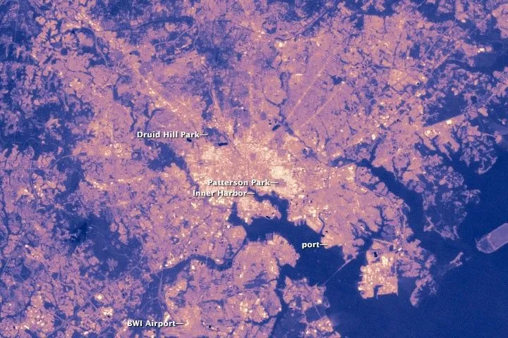
A satellite temperature map can show a hot industrial district while a nearby weather station reports a much lower temperature. Both observations may be correct. The satellite estimates the temperature of visible surfaces, while the station measures the air around its sensor. These measurements describe different parts of the urban environment and should answer different planning questions.
For cities assessing tree planting, cool roofs or neighbourhood heat, the practical challenge is choosing the right indicator, matching observations in time and space, and explaining what the results actually demonstrate.
Three Different Ways to Describe Urban Heat
Land surface temperature: how hot visible surfaces are
Satellite-derived land surface temperature, or LST, estimates the temperature of the surfaces contributing to the thermal signal received by the sensor. Depending on the location, these may include roofs, roads, bare soil, grass or the upper leaves of a tree canopy.
The instrument measures thermal-infrared radiation. Retrieving surface temperature requires accounting for atmospheric effects and surface emissivity—the efficiency with which a material emits thermal radiation. An uncorrected brightness-temperature image is therefore not automatically a land surface temperature product.
Our introduction to satellite thermal intelligence explains the broader principles and applications. For urban projects, the essential point is that LST describes the surface seen from above, including a mixture of materials within each thermal footprint.
Near-surface air temperature: how warm the air is
Weather stations measure air temperature using instruments protected from direct solar heating and exposed to ventilation. Sensors are commonly positioned approximately 1.25–2 metres above the ground, depending on the observing standard.
This measurement is affected by the surrounding environment, but it is not the temperature of the ground beneath the instrument. Nor does one station necessarily represent every street, park or industrial estate across a city.
Heat exposure: the conditions people experience
Human heat exposure also depends on humidity, wind and radiation. Two places with similar air temperatures can present different conditions for a person standing in direct sunlight or resting in shade.
The heat index combines air temperature and relative humidity and is intended for shaded conditions with light wind. Wet Bulb Globe Temperature, or WBGT, also accounts for wind and radiation and is used to assess heat stress during outdoor activity. Neither can be obtained simply by relabelling a satellite LST map.
Why Roofs, Roads and Green Spaces Differ from Weather Stations
Sunlight heats surfaces directly. How much they warm depends on their reflectivity, moisture, thermal properties and exposure. Vegetation can provide shade and evaporative cooling, while dry paved areas often have less moisture available for evaporation. Buildings also influence shade, ventilation and heat storage.
The air responds through heat exchange, mixing and movement. Consequently, there is no universal temperature offset that converts a roof or road temperature into the air temperature above it. The relationship changes with weather, surface conditions and time of day.
Three mismatches commonly complicate a comparison:
- Different measurement targets. A roof pixel and a sheltered air sensor measure different physical quantities, even when their locations are close.
- Different spatial support. A satellite footprint can contain roofs, trees, roads and shaded ground. A station samples air at one site, influenced by its surroundings and the airflow reaching it.
- Different observation times. A satellite snapshot cannot be compared directly with a daily maximum, daily mean or a temperature recorded several hours later.
Resolution also matters. Landsat 8 and 9 thermal measurements are acquired at 100-metre resolution and distributed on a 30-metre grid. Resampling does not create independent temperature measurements for every 30-metre patch. A small playground or individual roof may remain mixed with neighbouring surfaces.
A difference between satellite LST and station air temperature is not, by itself, evidence of satellite error. Validating LST requires suitable surface-temperature reference measurements, with timing, emissivity and measurement footprint addressed. Station air temperature is useful for interpreting weather conditions or evaluating a separate air-temperature model.
A Vancouver Example: Matching Imagery with Station Observations
Consider a project examining surface heat across Vancouver during June–August 2022. A practical approach would pair Landsat Collection 2 Level-2 surface temperature observations with hourly weather records from Environment and Climate Change Canada.
The following is a worked comparison design, not a completed analysis. It does not report measured temperature differences, correlations or cooling effects.
1. Select individual scenes before creating a seasonal map
Identify scenes covering the study area and retain their product identifiers, acquisition dates and acquisition times. Check whether surface temperature is available, then apply the product’s scale factor and offset before converting kelvin to degrees Celsius.
Screen clouds, cloud shadows and invalid observations using the quality information. Review cloud-adjacent areas and temperature uncertainty as well: USGS documents known surface-temperature retrieval problems near clouds and possibly cloud shadows. A low scene-wide cloud percentage does not guarantee that a particular neighbourhood is usable.
2. Match the time conventions explicitly
Use the acquisition time recorded in the scene metadata rather than an assumed overpass hour. Check whether station timestamps use UTC, local standard time or daylight-saving time.
Canadian surface-weather archives commonly use local standard time. Vancouver’s summer civil clock uses Pacific Daylight Time, one hour ahead of Pacific Standard Time. A mismatch can therefore pair the satellite observation with the wrong hourly weather record.
For illustration only, a timestamp of 19:00 UTC on a Vancouver summer date corresponds to 11:00 Pacific Standard Time and 12:00 Pacific Daylight Time. This is a time-conversion example, not the acquisition time of a selected scene.
Use the closest suitable station observation and record its time difference from the satellite acquisition. If interpolating between hourly records, state the method and avoid treating the interpolated value as a direct observation.
3. Check what the station represents
Vancouver International Airport offers an identifiable starting point for an hourly-record search. Before extracting data, confirm the station identifier, operating period, coordinates, elevation and availability for summer 2022.
Inspect the station setting and the surrounding satellite footprint. An airport station should not be assumed to represent a downtown street canyon, a wooded park or an inland industrial district. Additional stations or temporary sensors would be needed to examine those environments.
4. Extract surface observations without hiding mixed pixels
At the station location, inspect the containing pixel and a surrounding area appropriate to the thermal resolution. Record the land-cover mixture, valid-data coverage and the sensitivity of the result to the extraction area. A larger buffer is not automatically more representative.
Separately summarise larger urban zones—such as predominantly paved industrial areas, residential neighbourhoods and vegetated parks—using consistent boundaries and quality screening. Keep these zone summaries distinct from the station-site comparison.
5. Build one comparison record per accepted overpass
Each record should contain the scene identifier, acquisition time, station identifier, station observation time, time difference, extracted LST, air temperature, humidity, wind, relevant weather observations and quality flags. Recent rainfall and changes in surface cover should also be recorded where information is available.
Plot LST and air temperature as separate variables. If calculating their difference, label it “surface–air temperature difference,” rather than “satellite error.” Any fitted relationship should be tested on independent observations before being used to estimate air temperature elsewhere.
This design makes disagreement interpretable. It allows an analyst to investigate whether the contrast reflects surface heating, weather, station location, mixed pixels or retrieval uncertainty, instead of forcing two different measurements to agree.
A Summer Composite Is Not an All-Day Average
A single overpass describes surface conditions at one observation time. Combining several observations creates a different product, whose meaning depends on how those observations were selected and aggregated.
- Single-overpass LST: a snapshot of valid surface-temperature retrievals during one acquisition.
- Clear-sky seasonal mean LST: the mean of accepted observations during the selected season, usually within the satellite’s observation-time range.
- All-day mean surface temperature: a quantity requiring adequate sampling of the daily temperature cycle or an explicitly evaluated reconstruction method.
- Daily mean air temperature: a separate station or model statistic, calculated according to the dataset’s stated convention.
A summer composite of clear-sky daytime observations does not represent all weather conditions or all hours. Clouds restrict thermal-infrared surface observations, and different pixels may retain different dates after screening. A seasonal map should therefore include valid-observation counts and information about the dates contributing to each area.
A useful title would be “Mean Clear-Sky Daytime Land Surface Temperature, Vancouver, June–August 2022,” accompanied by the actual observation-time range and compositing method. “Average Summer Temperature” leaves too much room for misunderstanding.
Choose Indicators Around the Urban Decision
How to Evaluate Cooling Without Confusing Weather with Progress
A cooler image after an intervention does not establish that the intervention caused the change. The second acquisition may follow rainfall, occur under stronger wind or simply capture a cooler day.
Plan the evaluation before work begins. Record intervention boundaries and dates, select comparable untreated areas, and collect repeated observations before and after implementation. Keep sensor choice, processing, seasonal windows and surface classes consistent where possible.
One useful analysis compares how the treated area’s temperature contrast with a reference area changes over time. This can help account for shared weather variation, but it still requires checking whether the reference area remained comparable and unchanged. Report the result as a surface-temperature response unless air-temperature or exposure measurements support a broader conclusion.
Tree planting requires particular care. As canopy develops, a satellite may increasingly observe leaves rather than the ground beneath them. A cooler canopy signal is valuable information, but it does not directly quantify the conditions experienced by pedestrians below.
What a Useful City Heat Assessment Should Deliver
A decision-ready assessment should connect the map to follow-up work:
- Hot-surface locations: recurring warm areas, their dominant land cover and the spatial scale at which they can be interpreted.
- Comparable changes: repeated surface-temperature contrasts, with observation dates, weather context and intervention status.
- Evidence quality: valid-observation counts, retrieval uncertainty, cloud-related exclusions and areas affected by mixed pixels.
- Ground-observation priorities: locations requiring air sensors, surface measurements or radiation and humidity observations to answer the project’s remaining questions.
Satellite imagery provides the spatial view needed to identify recurring hot surfaces and guide field measurements. Ground observations then establish whether planned changes also improve air temperatures or conditions where people spend time.
STARPATH GLOBAL combines satellite resources, data processing and AI geospatial analysis to support urban and environmental monitoring. If you are planning a cooling assessment, discuss your project with our team to define the indicator, suitable thermal resolution and observation schedule, and the ground measurements needed to make the findings useful for city decisions.