Satellite imagery can reveal exposed salt crusts, identify crop patterns consistent with salt stress, and support soil salinity estimates calibrated against ground measurements. These are three different results. A bright patch of soil or a low vegetation index alone cannot establish how saline the soil is, particularly below the surface.
For agricultural monitoring, the useful question is what evidence supports the intended decision: locating areas for inspection, planning soil sampling, or estimating salinity across a defined soil depth. Each requires a different combination of imagery, field observations and validation.
Three Results That Need Different Evidence
1. Identifying Exposed Salt Crusts
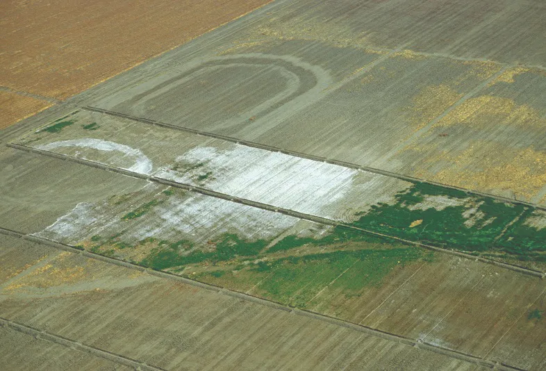
Where salts accumulate on bare ground, they can change surface brightness and spectral reflectance. Optical imagery may help delineate these deposits, especially when they cover enough of a pixel and are not obscured by vegetation, residue or wet soil.
However, white ground is not a diagnosis. Pale sand, carbonate-rich soil, exposed rock and other materials can produce similar appearances. A map derived from brightness alone should identify suspected surface deposits for inspection. Even a confirmed salt crust does not establish the salinity of the entire root zone.
2. Screening for Salt Stress Through Crops
Salinity can restrict plant water uptake and reduce growth. Satellite time series may reveal persistent areas of weak canopy development, uneven emergence or reduced vegetation cover that warrant investigation.
These responses are not specific to salt. Drought, waterlogging, nutrient deficiencies, pests, planting dates and management differences can produce similar patterns. Fallow land may also have a low vegetation index without being saline. Comparisons should account for crop type and growth stage, supported by irrigation, weather and field records.
3. Estimating Soil Salinity with Ground Data
Quantitative mapping requires a defined target, such as the electrical conductivity of a saturated soil paste extract, commonly written as ECe and reported in decisiemens per metre (dS/m). A model can relate that measurement to satellite observations and supporting environmental data.
The resulting map is a prediction calibrated to the sampled conditions. Optical imagery does not directly measure electrical conductivity or see through soil to the root zone. Any estimate for a subsurface layer depends on a demonstrated relationship between the observations and measurements from that depth.
Choosing Imagery for Bare Soil and Cropped Fields
For bare soil, select dates when the surface is exposed and document recent rainfall, irrigation and tillage. Moisture, soil texture, organic matter and residue affect reflectance and can obscure or imitate salinity-related patterns. A dry-season image may reveal surface deposits more clearly, but it should not be assumed to represent conditions throughout the year.
Landsat and Sentinel-2 provide useful multispectral observations for regional screening and repeated comparisons. Sentinel-2 includes visible, near-infrared, red-edge and shortwave-infrared bands, but their native resolutions differ. Its shortwave-infrared bands are acquired at 20 metres; resampling them to a 10-metre grid does not create independent 10-metre measurements.
For cropped fields, a time series is usually more informative than a single image. Repeated observations can distinguish recurring poor performance from an isolated event, although persistent drainage or management problems may still resemble salinity. Crop history and local measurements remain necessary to interpret the pattern.
Use analysis-ready reflectance products where appropriate, inspect quality flags, and apply the documented scale factors and offsets before calculating indices. A visually enhanced RGB image is useful for interpretation but does not replace calibrated spectral data.
Why Hyperspectral Band Coverage Matters
Hyperspectral imagery can provide more detailed spectral information, but the number of bands does not establish whether a sensor is suitable for salinity analysis. Check the wavelength range, band widths, signal quality, spatial resolution and usable bands after atmospheric correction.
A 2002 study in the Journal of Environmental Quality examined experimentally formed salt crusts across 400–2500 nanometres and identified absorption features associated with different crust materials. This demonstrates the value of spectral detail under controlled conditions; it does not mean that every feature is detectable from orbit or that crust composition directly gives root-zone salinity.
A sensor limited to visible and near-infrared wavelengths cannot capture shortwave-infrared features outside its range, regardless of how many bands it has. Conversely, broad shortwave-infrared bands do not resolve every narrow absorption feature. Data selection should follow the proposed method and local conditions, rather than the “hyperspectral” label alone.
What a Published Agricultural Study Shows
A 2015 study in Remote Sensing of Environment assessed soil salinity in California’s western San Joaquin Valley using seven years of Landsat 7 canopy reflectance, alongside crop-cover and meteorological information.
The researchers surveyed 22 fields covering 542 hectares. Electromagnetic induction measurements were calibrated against soil analyses from 267 locations to map salinity over the 0–1.2-metre root zone. Those maps provided reference data for the satellite model.
Validation held out one field at a time, giving an R2 of approximately 0.61. Mean absolute errors varied across salinity classes, from about 2.12 to 5.64 dS/m. These errors matter when distinguishing neighbouring classes or interpreting relatively low salinity.
The study demonstrates a route to regional estimation through canopy response, ground surveys and spatial validation. Its accuracy cannot be assumed for another region, crop system or sensor, and a multi-year model does not automatically establish short-term salinity changes.
A Workflow from Screening to Repeat Measurement
1. Define the Target and Screen the Imagery
Specify whether the project will map suspected crusts, prioritise salt-stress inspections or estimate a measured soil property. For quantitative work, define the sampling depth, measurement method and reporting unit before modelling. Use imagery and field records to identify contrasting surface, crop and drainage conditions.
2. Sample Across Those Conditions
Stratify sampling across suspected severity levels, soil types, irrigation zones and crop conditions. Include apparently unaffected areas and locations where the imagery is ambiguous. Sampling only obvious white patches would give a poor basis for estimating conditions across the wider landscape.
Record coordinates, collection dates, depth intervals, recent irrigation or rainfall, and surface condition. Match the sampled area to the satellite pixel as closely as practical; a single small soil core may not represent a mixed pixel containing crops, bare soil and a drainage ditch.
3. Measure Conductivity with a Consistent Method
Distinguish ECe from conductivity measured in a fixed soil-to-water extract, such as 1:5. Values from different extraction methods are not interchangeable without an appropriate conversion. Record the extraction procedure, temperature reference and units.
Field sensors measuring apparent electrical conductivity, ECa, can help guide sampling. Their readings also respond to water content, texture and other soil properties, so they need local calibration before being interpreted as salinity. Where salt composition or sodicity matters, request the relevant laboratory analyses rather than inferring them from imagery.
4. Validate Beyond the Training Samples
Reserve independent fields or spatial blocks for evaluation. Randomly splitting nearby samples can make performance appear stronger because training and validation locations share similar conditions.
Report bias and errors in the target unit, including performance across salinity ranges and land-cover conditions. If the output is a classification, report missed saline areas and false alarms. Identify areas outside the model’s sampled range and retain an uncertain category where the evidence is insufficient.
5. Repeat Measurements Before Claiming Change
Return to documented locations and depth intervals, using the same analytical method. Interpret repeat imagery alongside rainfall, irrigation, crop rotation and management records. Greener vegetation after rainfall or a change of crop does not, by itself, prove that salts have been removed from the root zone.
What a Useful Salinity Map Should Include
A reviewable delivery should show the study area, image dates, sampling locations, validation locations and areas excluded from analysis. Keep observed surface features separate from modelled soil values, and state the depth, measurement method, units, reference period and geographic limits of the estimates.
For a published case, present the imagery, sampling layout and validation results for the same study area, with their original attribution and reuse permissions. Where local samples are unavailable, deliver an inspection-priority map and sampling plan rather than assigning unverified conductivity values.
Satellite observations can help direct fieldwork and extend validated measurements across an agricultural landscape. Their value depends on keeping the conclusion matched to the evidence: visible deposits support surface interpretation, crop patterns support investigation, and calibrated models support estimates within their tested conditions.
For projects combining soil investigation with wider agricultural monitoring, STARPATH GLOBAL can help assess suitable data sources and observation timing. Compare spectral coverage and resolution in our imagery catalog, or discuss your project with our team to align imagery selection with the field measurements available.
Top image: Salinization—the buildup of salts in soils to levels that are harmful to plants—is a worldwide problem and affects about one-fourth of the irrigated land in the United States. White salt deposits, from severe salinization, coat fields in the western San Joaquin Valley in California.