In brief: Landsat and Sentinel-2 can capture flood details well, but they are most vulnerable to the very condition that often accompanies major flooding: cloud cover. Rather than trying to generate a visually plausible cloud-free optical image, this study directly reconstructs whether the surface beneath the clouds is water or non-water. The researchers combined Harmonized Landsat and Sentinel-2 (HLS) imagery, the Prithvi-100M foundation model, historical water-occurrence data from Global Surface Water, and a spatiotemporal Markov random field into a single workflow. The result turns 30 m optical flood maps from cloud-fragmented snapshots into a continuous time series. Across four global case studies, the method raised the average flood-period reconstruction F1 score from 0.871 to 0.931, with its advantage becoming more pronounced as cloud cover increased.
One of the greatest frustrations in optical flood monitoring is simple:
The heavier the rain and the more severe the flooding, the more clouds there are likely to be.
A satellite may pass over the same area every two or three days, yet only a small number of those observations may provide a clear view of the ground.
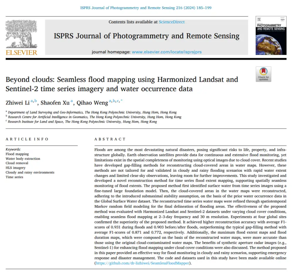
In 2024, Zhiwei Li, Shaofen Xu and Qihao Weng published a study in the ISPRS Journal of Photogrammetry and Remote Sensing titled:
Beyond clouds: Seamless flood mapping using Harmonized Landsat and Sentinel-2 time series imagery and water occurrence data
The study does not merely ask whether water-segmentation accuracy can be improved incrementally. It tackles a more difficult question:
If half—or even more—of an optical satellite image is obscured by clouds, can researchers still recover a spatially continuous flood map and assemble those maps into a continuous record of the event?
1. The Problem Is Not Just Cloud Cover—Floods Also Change Quickly
Missing observations of ordinary surface water can sometimes be filled using images acquired before and after the gap.
Floods are different.
A river can expand rapidly over a few days and then recede just as quickly. A dam failure can even produce two opposite changes at the same time: rapid downstream inundation and rapid water loss from the upstream reservoir.
That means a simple rule such as:
Yesterday’s water → today’s cloud-covered area
can easily produce the wrong result.
Conventional gap-filling may work for permanent lakes or seasonal water bodies. During a rapidly changing flood, however, the real problem is that conditions beneath the clouds may already differ completely from those observed in the previous image.
Synthetic aperture radar can observe through clouds, but the temporal density of openly available SAR data is also limited. At the time of the study, Sentinel-1B had ceased operations, leaving the remaining Sentinel-1 satellite with a revisit interval of about 12 days. That can still miss critical stages of a short-lived flood.
The researchers therefore chose a different route: use Landsat 8/9 and Sentinel-2 to build a high-frequency optical time series, then specifically address the flood information missing beneath clouds.
2. Why Is HLS Well Suited to This Task?
The study uses Harmonized Landsat and Sentinel-2, or HLS.
HLS applies consistent processing to surface-reflectance products from Landsat 8/9 and Sentinel-2A/B, making observations from different satellites easier to combine in a single time series.
The resulting data have two important characteristics:
- Spatial resolution: 30 m
- Typical observation interval: about two to three days
After the researchers combined Landsat and Sentinel-2 observations and retained partially cloud-covered images, the average observation intervals across the four study areas fell from:
- 8.3 days to 3.1 days
- 5.0 days to 2.5 days
- 6.2 days to 3.2 days
- 4.4 days to 2.9 days
HLS therefore addresses the first question:
How often does a satellite return?
The cloud-reconstruction method addresses the next one:
What happens when the satellite returns but clouds block the ground?
Only by solving both problems can optical imagery support a genuinely high-density flood time series.
3. The Workflow Has Three Main Steps: Detect Water, Fill Cloud Gaps and Let the Time Series Correct Itself
The workflow shown in Figure 1 on page 3 of the paper is straightforward.

Step 1: Prithvi-100M Extracts Water From Each Image
Each HLS image is first processed by a fine-tuned foundation model to produce an initial map with three classes:
- Water
- Non-water
- Cloud-shadow
Step 2: Historical Water Occurrence Is Used to Reconstruct Cloud-Covered Areas
For areas obscured by clouds or cloud shadows, the method does not simply copy the preceding image. Instead, it uses water occurrence from the Global Surface Water (GSW) dataset to estimate how likely water has historically been at each location.
The authors also introduce a “submaximal stability” assumption to determine a local water-occurrence threshold automatically.
Step 3: A Spatiotemporal MRF Refines the Results
Even after reconstruction, isolated errors may remain between dates.
The researchers use spatial neighborhoods and consistency across adjacent time steps to make a further correction, producing water patterns that are more spatially connected and temporally plausible.
The full process can be summarized as:
Single-image detection → cloud-area inference → spatiotemporal consistency refinement
Compared with simple interpolation beneath clouds, this approach adds a constraint based on the dynamics of the flood itself.
4. Prithvi-100M Plays a Simpler Role Than Its Name Might Suggest
The study uses Prithvi-100M, a foundation model developed by NASA and IBM.

Prithvi-100M is a remote-sensing foundation model based on a Vision Transformer and masked autoencoder architecture. It was pretrained on a large volume of HLS imagery.
The study uses six optical bands:
- Blue
- Green
- Red
- Narrow NIR
- SWIR 1
- SWIR 2
The authors further fine-tuned the Prithvi-100M–Sen1Floods11 architecture for single-image water segmentation.
The 446 labeled chips in Sen1Floods11 were divided into:
- 267 for fine-tuning
- 89 for validation
- 90 for testing
The fine-tuned model achieved the following results:
Prithvi does not directly infer the entire flood time series in this study.
Although the Prithvi architecture itself can support multitemporal modeling, the researchers use it here to extract water from individual HLS observations. Most of the temporal information enters later through cloud reconstruction and the MRF.
The study’s innovation is therefore not that a large model directly predicts flood evolution.
5. The Central Challenge: How Can Historical Water Occurrence Reveal Whether Water Is Beneath Today’s Clouds?
The researchers use the water-occurrence layer in GSW.

Derived from Landsat observations collected between 1984 and 2021, the layer can be understood as the percentage of valid historical observations in which a given pixel was classified as water.
For example:
- 90%: water has appeared very frequently over the long term
- 50%: the location may contain seasonal water
- 5%: water has rarely appeared there in the past
The simplest possible approach would be:
High historical water occurrence → classify the cloud-covered pixel as water
But floods often spread into areas where water has historically occurred only rarely.
If the threshold is too high, the method will miss real inundation. If it is too low, large areas of land will be incorrectly reconstructed as water.
The authors therefore propose the submaximal stability assumption.
In plain language, the method does not blindly trust a fixed water-occurrence value. It first examines the relationship, within the currently visible cloud-free area, between historical water occurrence and the water actually detected on that date. It then determines an appropriate threshold for the local area.
This changes the threshold from a single global value into a locally adaptive one.
6. How Does “Submaximal Stability” Work? The Key Is Not 0.35, but Finding a Reliable Local Range First
The method can be simplified into three steps.
First, it establishes a local window around the target pixel. The initial window size is:
50 × 50 pixels
If the window does not contain enough valid cloud-free pixels, it expands progressively.
The method then calculates two water-occurrence histograms:
- Water occurrence for all pixels in the currently valid area
- Water occurrence for pixels currently identified as water
It then calculates, within each water-occurrence bin:
Number of pixels currently identified as water / number of all valid pixels
This ratio can be interpreted as:
Among pixels with this level of historical water occurrence, what proportion actually appears as water today?
As water occurrence rises, the ratio generally increases and begins to stabilize.
Based on a sensitivity analysis, the authors ultimately set:
Pixel count ratio = 0.35
as the decision threshold.
Once the method finds the first bin in which the ratio exceeds 0.35, the corresponding water-occurrence value becomes the reconstruction threshold, T, for that local window.
Finally:
Cloud-covered pixel with water occurrence > T → reconstruct as water; otherwise → reconstruct as non-water
The value 0.35 therefore does not mean “35% water occurrence.”
It is the pixel-count ratio used to identify the local water-occurrence threshold.
The two concepts should not be confused.
7. Why Is a Local Window Better Suited to Floods Than a Global Threshold?
Flood behavior is highly heterogeneous across space.
Upstream areas may experience only slight river expansion. The middle reaches may see extensive floodplain inundation, while downstream conditions may be altered by lakes or reservoirs.
In the Michigan dam-failure case, reservoir water contracted at the same time that flooding expanded downstream.
A single global water-occurrence threshold for the entire image would struggle to represent all of these changes.
The paper’s local sliding window continually adjusts the threshold according to nearby valid pixels.
In effect, each local area uses its own combination of current visible water conditions and historical water patterns to decide how cloud-covered pixels should be reconstructed.
The tradeoff is clear:
It requires more computation.
The authors nevertheless found that the resulting local adaptability produced a substantial improvement in accuracy.
8. The MRF Does Not Simply Perform Another Classification—it Makes Adjacent Dates Check One Another
Abrupt inconsistencies can remain after cloud-covered areas have been reconstructed.
For example, a pixel might be classified as:
Water in the preceding image → suddenly non-water in the current image → water again in the next image
If the flood could not plausibly have changed that quickly, the middle classification deserves scrutiny.
The authors apply a spatiotemporal Markov random field, or MRF, to refine the result.
It uses:
- A spatial neighborhood of 3 × 3 pixels
- Five adjacent time steps before and five after the current time step
- Weights based on spatial and temporal distance
- An optimization process that seeks a lower-energy, more neighborhood-consistent water or non-water state
The method also does not treat reconstructed pixels as equally reliable as genuine cloud-free observations.
Reconstructed pixels receive a weight of only:
0.75
In other words, an inferred result beneath a cloud can contribute to the time-series assessment, but it is trusted less than a pixel the satellite actually observed.
The experiments also show that the MRF becomes more valuable as cloud cover increases.
9. The Four Cases Were Chosen to Create Different Types of Difficulty
The paper examines four flood events.

Assam, India
Flooding from May to August 2022. Heavy cloud cover and a long-lasting event make this a representative monsoon-flood case.
Sindh, Pakistan
Flooding in August and September 2022. The affected area was extremely large, but cloud cover was relatively low during some stages, making it useful for testing high-frequency HLS mapping.
Rio Grande do Sul, Brazil
Flooding in October 2023. Heavy cloud cover and limited valid observations make this a genuinely difficult case in which optical information is scarce.
Michigan, United States
Dam-failure flooding on May 19, 2020.
Unlike the first three cases, not all water bodies expanded. Reservoir levels fell while new flooding developed downstream.
This tests whether the method can handle a complex pattern in which some places become wetter while others simultaneously become drier.
Together, the four cases test different cloud conditions, flood types and water dynamics.
10. The Main Result: The More Cloud There Is, the Greater the Advantage Over Conventional Gap-Filling

The researchers created reference water maps from genuinely cloud-free HLS imagery and then superimposed real cloud masks to simulate three levels of obstruction:
- Low cloud cover: <30%
- Medium cloud cover: 30%–60%
- High cloud cover: >60%
Because the underlying cloud-free observation was known, the researchers could quantitatively determine what was actually beneath the simulated clouds.
During Floods
Average F1 score for conventional gap-filling:
0.871
Average F1 score for the complete method:
0.931
Before and After Floods
Average F1 score for the conventional method:
0.772
Average F1 score for the proposed method:
0.903
The results by cloud level are even more revealing.
The complete method achieved overall average F1 scores of approximately:
- Low cloud cover: 0.955
- Medium cloud cover: 0.920
- High cloud cover: 0.875
Absolute accuracy still declined as cloud cover increased, but the method’s advantage over the comparison approach became larger.
Under high cloud cover, the F1 improvement reached:
0.140
The method does not eliminate the uncertainty caused by clouds. Rather, it becomes less likely than conventional gap-filling to fail as cloud conditions worsen.
11. How Much Does the MRF Contribute? Its Value Is Much Greater Under Heavy Cloud Cover
The authors also compared:
Cloud reconstruction only
with:
Cloud reconstruction + MRF spatiotemporal refinement
The absolute F1 gains produced by the MRF under low, medium and high cloud cover were approximately:
- 0.016
- 0.033
- 0.071
In other words, the more cloud cover there is—and the less reliable any single image becomes—the more important neighboring observations in the time series become.
This is intuitive.
If 80% of an image is obscured, the remaining 20% of visible ground provides too little information to reconstruct the entire flood confidently. The flood’s trajectory in the preceding and following images then becomes critical evidence.
But this also reveals an important operational limitation.
The paper’s MRF uses five time steps before and five after the current image.
It therefore relies on future imagery to refine the map for the current date.
The complete method is consequently better suited to flood-event reconstruction, near-real-time updating with some delay, or operational products that tolerate latency.
If a user requires a final map immediately after the satellite passes overhead, the five future observations do not yet exist. The MRF would need to use historical observations only or be replaced with another online update mechanism.
This distinction is essential when interpreting “high temporal resolution” and genuinely real-time performance.
12. What Do PlanetScope, Maximum Flood Extent and Flood Duration Each Demonstrate?
The study also uses 3 m PlanetScope imagery for validation.

The authors explicitly state, however, that PlanetScope can be used only for visual validation.
PlanetScope and HLS imagery are not always collected at the same time. Cloud conditions and flood boundaries may already have changed, so PlanetScope cannot serve as strict pixel-by-pixel ground truth.
Two derived products provide more useful evidence:
- Maximum flood extent
- Flood duration or occurrence-frequency map
Compared with maps produced directly from the original cloud-contaminated water observations, the reconstructed time series more completely captured the maximum inundation extent and reduced the large number of spatial gaps in the flood-duration map.
This shows that filling cloud gaps is not merely about making an individual map look complete.
The greatest benefits appear in estimates of the flood’s maximum footprint, duration and evolution over time.
13. Why Did Adding Sentinel-1 Improve the Result by Only 0.12%? The Small Gain Is Itself Important
The researchers also tested adding Sentinel-1 water maps to the HLS time series.

In theory, SAR should be highly valuable because it can observe through clouds.
In practice, however, it improved the F1 score by only about:
0.12%
That gain is extremely small.
The reason is not that SAR lacks value. It is that SAR and optical sensors do not observe water through the same physical mechanisms.
Even on the same day, the water boundaries derived from optical imagery and Sentinel-1 can differ substantially.
SAR measurements are affected by surface roughness, vegetation, buildings, incidence angle and scattering mechanisms. Optical observations are affected by clouds, shadows and spectral mixing.
Figure 10 on page 13 of the paper shows clear spatial differences between same-day SAR and HLS water results.
The authors therefore take a cautious position:
SAR has considerable potential as a supplementary data source under heavy cloud cover, but effective joint optical-SAR flood mapping first requires harmonization between the two types of water product.
The paper should therefore not be described as having already achieved seamless optical-SAR fusion.
Here, SAR is primarily an extension experiment and a direction for future work.
14. Where Does the Study’s Real Innovation Lie?
The study’s value does not come from any one model alone. It comes from connecting several layers of information.
First, a foundation model improves water extraction from individual images.
Prithvi-100M is used to classify the optical observations in which the ground is actually visible as accurately as possible.
Second, the method reconstructs water or non-water status rather than attempting to recreate the optical image itself.
That is much simpler than generating realistic RGB values or spectral reflectance beneath the clouds, and it aligns more directly with the operational objective of flood mapping.
Third, the workflow uses historical water occurrence as prior knowledge without mechanically applying a fixed threshold.
The submaximal stability assumption and local window allow historical water probability to be interpreted dynamically according to current flood conditions.
Fourth, the MRF adds spatial and temporal continuity as a final quality-control step.
A reconstructed pixel is not evaluated in isolation. It must also be checked against neighboring pixels and adjacent observations.
The full framework can therefore be summarized as:
AI handles the places that can be seen, historical knowledge handles the places that cannot, and the spatiotemporal process performs the final correction.
Conclusion: Optical Flood Monitoring May Not Need to Reconstruct the Image Beneath the Clouds—Only the Water State
The study’s most memorable idea is also its most direct:
For flood operations, users do not necessarily need the true reflectance value of every spectral band beneath the clouds. In many cases, they need only a reliable answer to one question: Is this location currently water or non-water?
The researchers therefore avoid a complex generative cloud-removal approach and instead reformulate the problem as:
Cloud-contaminated HLS → extract visible water → infer cloud-covered areas using historical GSW water occurrence → refine the result with a spatiotemporal MRF
The method raises the flood-period F1 score from 0.871 for conventional gap-filling to 0.931. Under high cloud cover, its advantage reaches 0.140. The reconstructed time series also produces more complete maps of maximum flood extent and flood duration.
But the study also makes an important limitation clear:
Historical water probability is good at recovering water in places where it has occurred frequently before. By design, it is less capable of inferring an extreme flood that extends far beyond historical experience.
The most sensible next step is therefore not to rely ever more heavily on historical occurrence. As the authors propose in their conclusion, the approach should instead combine:
Optical imagery + SAR + high-resolution DEMs + hydrodynamic modeling + multitemporal foundation models
That would move the analysis beyond:
Does this location look like somewhere water has historically occurred?
and toward:
Given current rainfall, terrain and flood evolution, is flooding at this location physically plausible now?
Direct Implications for Flood Remote-Sensing Research
The following points are extensions of the paper’s framework, not experiments completed in the original study.
First, GSW water occurrence could be expanded from the sole historical prior into a multisource background model that includes seasonal water probability, Height Above Nearest Drainage (HAND), distance to river networks, historical flood frequency and hydrodynamic-model extents. This could reduce the risk that historically low water occurrence suppresses the detection of an extreme flood.
Second, the MRF demonstrates the importance of temporal continuity, but a genuine emergency system should replace the bidirectional time window with an online process that uses only past and current observations. Once the event ends, future observations could be incorporated in an offline reanalysis.
Third, the 0.12% improvement from adding SAR does not show that SAR is unhelpful. It shows that multisource fusion is not simply a matter of adding another dataset. The first task is to reconcile how different sensors define water and how their error structures differ. Future systems could assign separate confidence levels to optical observations, SAR observations and model estimates before combining them through weighted fusion.
Fourth, the final product should ideally provide more than a binary flood or non-flood label. It should also distinguish among:
- Direct optical observation
- Cloud-area reconstruction
- SAR supplementation
- Model inference
- Pixel-level confidence
This would allow users to distinguish between flooding the satellite actually observed and flooding inferred from historical and spatiotemporal information.
For organizations developing flood-monitoring or disaster-response workflows, STARPATH GLOBAL can help match optical and radar satellite imagery to the resolution, revisit frequency and budget a project actually requires, avoiding the cost of purchasing data that exceed operational needs. China’s expanding Earth-observation capacity is also making competitively priced imagery more accessible to international users; teams can contact STARPATH GLOBAL to evaluate suitable data options and explore the company’s imagery catalog. Organizations without in-house remote-sensing experience can also apply to the Pioneer Partner Program to work with STARPATH GLOBAL’s FDE team on use-case validation, workflow development and staff training.
Paper Information
Title: Beyond clouds: Seamless flood mapping using Harmonized Landsat and Sentinel-2 time series imagery and water occurrence data
Authors: Zhiwei Li, Shaofen Xu and Qihao Weng
Journal: ISPRS Journal of Photogrammetry and Remote Sensing
Volume and pages: Volume 216 (2024), pages 185–199
Published online: August 7, 2024
DOI: 10.1016/j.isprsjprs.2024.07.022
Core datasets: HLS Landsat 8/9 + Sentinel-2, GSW water occurrence, PlanetScope and Sentinel-1
Core models: Prithvi-100M–Sen1Floods11 and a spatiotemporal MRF
Four case studies: Assam, India; Sindh, Pakistan; Rio Grande do Sul, Brazil; and Michigan, United States
Spatial and temporal scales: 30 m, with combined observations approximately every two to three days